Math/Art

William Worden Home Research Teaching CV

This page is under construction : )

Seifert--Weber dodecahedral space, icosahedral manifold

The polyhedral decomposition of the figure-8 knot into two tetrahedra. The fact that this is shaped like a tetrahedron does nothing to help you see why the polyhedra are tetrahedra, but it looks cool! Same as the previous slide, but with a couple of faces removed to make it easier to see what's going on. The polyhedral decomposition with the yellow bigons (see previous set of slides). Decomposition with yellow bigons, with some faces removed.

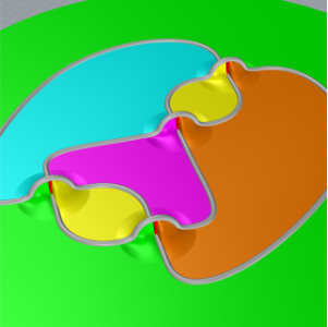
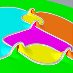
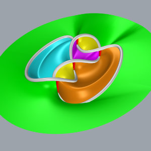
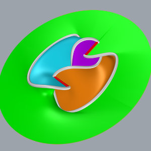
Thurston's tetrahedral arrangement of the figure-8 decomposition

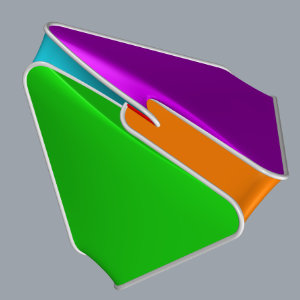
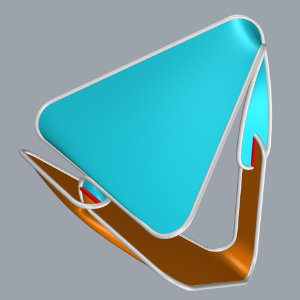
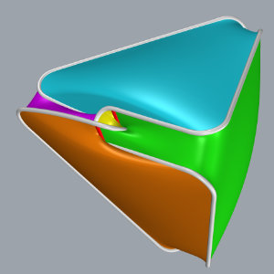
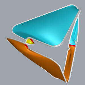
In Three-Dimensional Geometry and Topology, Thurston describes another way to construct the decomposition of the figure-8 knot complement from above. First we draw the figure-8 knot so that it sort of looks like a tetrahedron, then add faces. This is described on pages 40-43 of the book referred to. Here are some 3D models of what Thurston is describing.

The polyhedral decomposition of the figure-8 knot into two tetrahedra. The fact that this is shaped like a tetrahedron does nothing to help you see why the polyhedra are tetrahedra, but it looks cool! Same as the previous slide, but with a couple of faces removed to make it easier to see what's going on. The polyhedral decomposition with the yellow bigons (see previous set of slides). Decomposition with yellow bigons, with some faces removed.

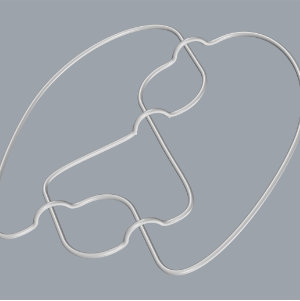
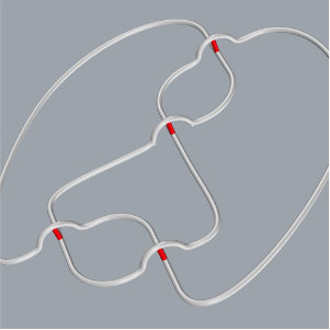
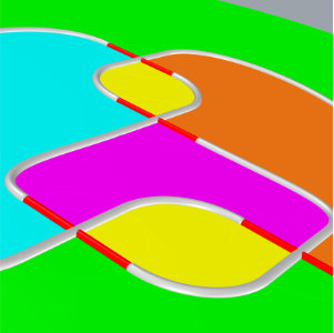
Polyhedral decomposition of the figure-8 knot complement

A knot is an embedding of a circle in 3-dimensional space (or in the 3-sphere). Intuitively, you can think of a knot as a tangled up extension cord, with the ends plugged together. It is often useful to study knots by understanding the space around the knot (not including the knot itself). To study the space around the knot, it is useful to break it up into simple polyhedral pieces. There is a recipe that gives a way to decompose the space around any knot into polyhedra, first demonstrated by Thurston in his 1979 notes for the figure-8 knot. A good source for details is the first chapter of Purcell's book Hyperbolic Knot Theory (also available on arXiv). The 3D models below demonstrate Thurston's decomposition.

The figure-8 knot Another view of the figure-8 knot. I've pulled it around (i.e., <em>isotoped</em> it), so that it lies in the plane as much as possible, and just jumps over itself at crossings. The first step in the polyhedral decomposition is to add an edge (red) at each crossing. Next we add faces in each portion of the plane bounded by edges and knot strands. The green face goes off to infinity in all directions. These faces cut the space into the half on the other side of all the faces, and the half on this side. Each of these halves is a polyhedron, though some of its edges have been folded together. To see it more clearly we'll need to unfold these edges . 
			Unfolding the pinched together edges of the polyhedron. This shows the unfolding for the polyhedron above the plane (the one we're in). The knot has been split into 4 strands (remember the knot isn't part of the space we're decomposing, so this is ok). Next we'll contract the knot strands to vertices, and stretch out the edges. The knot strands become vertices of the polyhedron. As they contract, the edges stretch. Now we have a graph in the plane. If we add the point at infinity to 3-dimensional space, then it becomes a 3-dimensional sphere, and the plane become a 2-dimensional sphere. So with this addition, we can think of this as a graph on a 2-sphere, which is a polyhedron. Note that some of the faces of the polyhedron are bigons (they have just two edges). These can be collapsed to get a polyhedron without bigons. A less flattened out version of the figure-8 knot decomposed into polyhedra. Here I have collapsed the bigons. Now the two polyhedra in the decomposition are tetrahedra (each has 4 triangular faces).

GH Calculus Tools

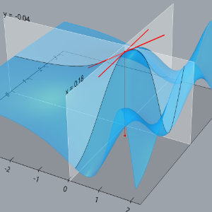
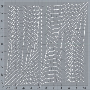
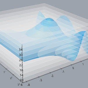
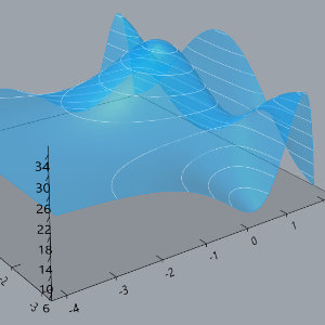
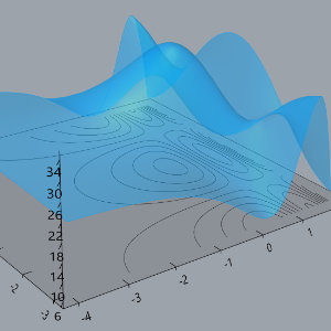
Some tools for visualizing multi-variable calculus concepts, programmed in Rhino3D/Grasshopper. Files are on GitHub here.

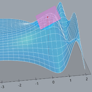
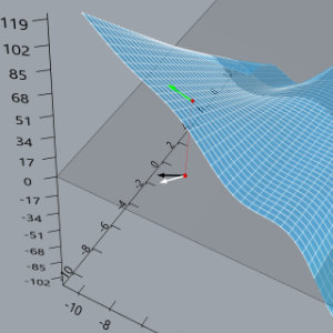
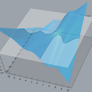
The main tool is surface_plotter.gh, which is an interactive 3D graphing calculator that has features that were added in the course of teaching a multi-variable calculus course to visualize things like cross-sections of surfaces, partial and directional derivatives, contour plots, gradients, etc. The other files include tools for visualizing quadric surfaces and parametric curves (and concepts surrounding them).

Using these files of course requires Rhinocerous, which is a closed-source 3D modelling program. These tools were developed for my own use, but I hope others will be able to make use of them as well. It is unfortunate, but unavoidable, that Rhino is not free, so there is a built in barrier here for access. However, Rhino offers a 90-day trial (and reduced pricing for educators), so that is an option to consider if you want to try this out.

XY traces tangent planes directional Z trace gradient field level planes level curves on surface contour plot